In Business Roundtable v. SEC, 1 647 F.3d 1144 (D.C. Cir. 2011). the D.C. Circuit struck down Rule 14a-11, which granted certain shareholders the right to nominate directors on the corporate proxy. 2 Id. at 1146. The decision is important not only because it halted the SEC’s efforts to regulate proxy access, but also because it imposes a new requirement of cost-benefit analysis for financial regulation.
In the Dodd-Frank Wall Street Reform and Consumer Protection Act (Dodd-Frank), Congress authorized the SEC to adopt Rule 14a-11. 3 Pub. L. No. 111-203, § 971, 124 Stat. 1376, 1915 (2010) (codified as amended at 15 U.S.C. § 78n (2012)). The court discovered the cost-benefit analysis requirement in language from a 1996 statute which directs the SEC to “consider, in addition to the protection of investors, whether [an] action will promote efficiency, competition, and capital formation.” 4 Business Roundtable, 647 F.3d at 1148 (citing 15 U.S.C. § 78c(f)). The D.C. Circuit reviewed the record and concluded that the agency’s analysis had failed to give sufficient weight to a single report prepared in support of comments submitted by the Business Roundtable during rulemaking. 5 Id. at 1149-51.
The new rule announced in Business Roundtable has generated a lively debate on the merits of cost-benefit analysis in finance. Robert Ahdieh argues that the 1996 statute demands some cost-benefit analysis, but does not require the SEC to adopt only rules that satisfy a particular cost-benefit standard. He suggests that the D.C. Circuit erred in Business Roundtable by reviewing the SEC’s conclusions on the merits.
6
Robert B. Ahdieh, Reanalyzing Cost-Benefit Analysis: Toward a Framework of Function(s) and Form(s), 88 N.Y.U. L. Rev. 1983, 2055-65 (2013).
Both John Coates and Jeffrey Gordon assert that precise cost-benefit analysis of capital markets regulation is a practical impossibility,
7
John C. Coates IV, Cost-Benefit Analysis of Financial Regulation: Case Studies and Implications 88-95 (Harvard Univ. John M. Olin Ctr. for
Law, Econ. & Bus., Discussion Paper No. 757, 2014), available at http://papers.ssrn.com/sol3/papers.cfm?abstract_id=2375396; Jeffrey N. Gordon, The Empty Call for Benefit-Cost Analysis in Financial Regulation 6-10 (Columbia Law Sch., Ctr. for Law & Econ. Studies Research Paper Series,
Paper No. 464, 2013), available at http://papers.ssrn.com/sol3/papers.cfm?abstract_id=2375396.
while Eric Posner and Glen Weyl argue that financial regulation cost-benefit analysis is simple in theory.
8
Eric Posner & E. Glen Weyl, Benefit-Cost Paradigms in Financial Regulation 1 (Coase-Sandor Inst. for Law & Econ., Working Paper No.
660, 2013), available at http://papers.ssrn.com/sol3/papers.cfm?abstract_id=2346466.
The debate over cost-benefit analysis for financial regulation is significant; Dodd-Frank directs regulators to adopt 398 new rules.
9
See David Zaring, Dodd-Frank Is Indeed Taking Root, N.Y. Times DealBook (Nov. 1, 2013, 1:04 PM),
http://dealbook.nytimes.com/2013/11/01/dodd-frank-is-indeed-taking-root. Also, agencies are directed to conduct 87 studies, which may spawn more rulemaking. See id.
So far, the debate has concentrated on whether economists understand finance well enough to determine the effect of a rule before its implementation. But the debate has ignored the more obvious conclusion from Business Roundtable. Science presents an interpretive challenge, one that judges are evidently ill equipped to handle. By replacing the SEC’s judgment with its own misinterpretation, Business Roundtable highlights a pervasive problem that the courts confront: scientific evidence is often conflicting, even if the weight of the evidence supports one consensus. As the number of empirical studies on a particular subject increases (and a consensus emerges), the number of individual studies that contradict the consensus tends to increase.
When a study produces a contrary result, it is often presumed to contain a flaw in the data or methodology. But contrary results are not always the product of flaws. Instead, good studies using good data will sometimes produce an unusual result because of statistical sampling.
This Essay illustrates the problem for both discrete and continuous variables, noting that the underlying distribution can complicate the analysis. After introducing a tangible example, the Essay proposes how to respond to the problem of contrary evidence.
Counting Marbles, or Discrete Variables
In the simplest illustration, the response variable is discrete. Consider the archetypal urn containing black and white balls. The ratio of black balls to white balls is unknown and a census is impractical: counting every ball would take too long. Instead, a sample is taken from the urn and the ratio of black to white balls is estimated. A very small sample tells us very little. Larger samples allow us to estimate the ratio with increasing confidence. For every sample smaller than the entire population, variation of the sample mean from the population mean is expected. Thus, if earlier samples suggest that black balls predominate white balls by nine to one, then finding slightly more or fewer should not be understood as disproof of our earlier conclusions.
10
Finding 87 black balls in a sample of 100 from a large population should not motivate doubt that 90% of the balls are black. If b is the
share of black balls in the sample and β is the share of black balls in the population, then finding that b is 0.87 should not be understood as
disconfirming that β is 0.90. In fact, observing that b is within 3% of the true value is some evidence that β is indeed 0.90.
Our confidence in our estimate of the mix increases as the size of the sample increases. Even though more white balls are found in a sample of one thousand than in a smaller sample, we are more confident that black balls predominate by nine to one. Only the most inept (or motivated) decisionmakers would interpret the increasing number of white balls in larger samples as contrary evidence, since the number of black balls is that much greater.
Less often, studies do not conduct a preordained number of trials, but instead keep sampling until a preordained number of results is reached.
11
The negative binomial distribution is a discrete probability distribution of the number of successes in a sequence of Bernoulli trials before a
specified (nonrandom) number of failures occurs. A Bernoulli trial is an experiment with two possible outcomes.
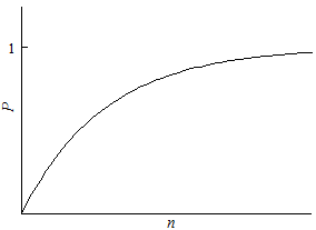
For example, we might want to know how many studies must be conducted before chance dictates a contrary result, allowing the decisionmaker to find a lack of consensus. Instead of sampling one hundred balls, the study might sample until five white balls are found. The likelihood of finding a ball of a particular color increases with the sample size. Figure 1 shows the probability of finding at least one white ball as the sample size increases. In a sufficiently large sample, the probability approaches certainty. The likelihood increases even as larger samples generate more confidence that white balls are rare.
If one color predominates, the likelihood of finding one color over another departs from even odds (or p = 0.5). Developing information about the underlying ratio takes longer if one color predominates.
12
The Kullback-Leibler divergence describes how quickly information accumulates to allow us to distinguish between two probability distributions.
Consider two urns, each with a different color ratio. Instead of sampling the urns to determine the color ratio, the color ratio is known, but the urn is
not. Therefore, sampling can determine which urn is being sampled by observing the color ratio in the sample.
It will take more samples to develop confidence in the ratio, suggesting that the scenarios which we imagine to be clear-cut will actually appear less so.
Figure 1
Estimating Coefficients, or Continuous Variables
The same effect exists when the response variable is continuous. Consider a relationship Y = ƒ(X). While we might hope to determine ƒ with accuracy and precision, often scholars merely hope to determine whether a relationship exists at all. Many legal questions present such methodological challenges that determining whether a relationship exists at all is a great achievement.
13
For example, some studies have found that capital punishment decreases crime, while others have found the opposite. Compare Hashem Dezhbakhsh
et al., Does Capital Punishment Have a Deterrent Effect? New Evidence from Postmoratorium Panel Data, 5 Am. L. & Econ. Rev. 344, 368-70 (2003)
(finding that each execution deterred, on average, eighteen homicides, with a margin of error of ten), with William J. Bowers & Glenn L.
Pierce, Deterrence or Brutalization: What Is the Effect of Executions?, 26 Crime & Delinq. 453, 471-77 (1980) (finding that executions
increase the homicide rate), and Lawrence Katz et al., Prison Conditions, Capital Punishment, and Deterrence, 5 Am. L. & Econ. Rev.
318, 326-39 (2003) (finding no deterrent effect).
Consider the simplest ƒ, a linear relationship we can write as Y = αX. Estimates should fall around the true value of α, but we can expect many to be higher or lower. If the samples are unbiased, half of the estimates should fall below and half above. We should not be surprised if some of the estimates of α fall far enough away from its true value that the sign is reversed, suggesting the opposite relationship between the variables.
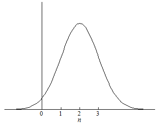
Assume the value of α is 2. As the value of X increases, the value of Y increases, but twice as quickly. In common parlance, the relationship is positive. If the samples are unbiased, half of the estimates for α will be larger than 2 and half will be smaller. If the standard deviation of α is 1,
14
The standard deviation is a measure of dispersion of the data. Larger standard deviations correspond to more spread out data. Here, the data is
assumed to be normally distributed. Other distributions present different interpretive challenges beyond the scope of this Essay.
we expect 68% of estimates to be between 1 and 3, as shown in Figure 2. In fact, assuming the same standard deviation, we can expect 2% of the estimates to fall below zero, suggesting the relationship is negative rather than positive. If the distribution is more dispersed, more of the estimates will fall farther from the mean value.
Figure 2
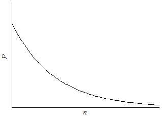
As the sample size increases, our confidence that the value of α is 2 increases. Like before, the likelihood of contrary evidence increases with sample size. Sufficiently large samples are almost certain to include values far from the mean. Since 95% of estimates will fall within two standard deviations of the mean, an estimate greater than two standard deviations is rare. In Figure 3, the likelihood that every estimate falls within a standard deviation of the population mean falls as the number of samples increases. As the sample size increases, the likelihood of no contrary evidence approaches zero. In other words, as the sample size increases, the number of contrary results will increase.
Figure 3
Interpretive Problems
The absolute number of contrary results is not as important as the relative share. Considering the relative number of contrary results is one way to prevent mistakes. An increasing relative share of contrary evidence, however, is not dispositive, since the relative share may increase as the sample increases in size while still remaining low. Both the absolute number of contrary results and the relative share provide information, but neither will provide definitive answers.
For example, the developing consensus on global climate change shows both the importance of the relative share over the absolute number of contrary results, while showing that an increasing relative share by itself is not good evidence. In 2004, Naomi Oreskes examined the 928 refereed articles addressing climate change published between 1993 and 2003, and found that 75% of them accepted the contention that humans have caused rising temperatures, while the remaining 25% took no position.
15
Naomi Oreskes, The Scientific Consensus on Climate Change, 306 Science 1686, 1686 (2004).
In 2012, James Powell found 13,950 refereed articles on global climate change; of that number, 24 articles reject the consensus position that the global climate is warming and human activity is the cause.
16
Original Study, James Lawrence Powell, http://jamespowell.org/Original%20study/originaltsudy.html (last visited Apr. 23,
2014).
Between 2004 and 2012, the number of studies rejecting human-caused climate change increased from 0 to 24. Between 2004 and 2012, both the absolute number of studies rejecting the consensus and their relative share increased. By 2012, there was significantly more contrary evidence, yet the scientific consensus was even stronger. Why? The number of studies concluding that human activity is warming the global climate increased from 696 to 13,926, and the relative share of contrary evidence increased from zero to only two studies per thousand.
To determine the number of studies rejecting the scientific consensus, Oreskes and Powell had to define the population of studies to be considered. If every study were identical, it would be trivial arithmetic to determine the absolute number and relative share of contrary results. More typically, studies are dissimilar, making purely numerical comparisons of absolute and relative figures impossible. Constructing the space of relevant studies requires judgment and that judgment is what determines the end result, not the arithmetic of comparing absolute and relative figures.
When studies are heterogeneous, comparing the relative share of contrary results is difficult and judicial mistakes are more likely. In fact, it is very difficult to tell when the reliance on contrary results is an honest mistake or not. Some administrative decisionmakers are not experts, especially political appointees who may have a stronger political than technical pedigree. Judges are not selected for their expertise in any field except law. Without expertise, it is difficult for judges to determine which studies are relevant, which are persuasive, and how to weigh the relative merits to reach a conclusion.
Even where the consensus is overwhelming, the methodology of discerning the scientific consensus is subject to criticism. The methodology used by Oreskes to determine that no papers challenged the global climate change consensus was criticized, although her conclusions were not called into question. Roger Pielke argued that Oreskes did not capture the full range of scientific opinion.
17
See Roger A. Pielke Jr., Letter to the Editor, Consensus About Climate Change?, 308 Science 952, 952 (2005).
Evaluating scientific papers to determine whether those papers fit into one of two categories is fraught, since the findings, arguments, caveats, and linguistic hedges resist binary classification. Given the methodological difficulties in determining into which of two categories a particular study should be classified, recent studies have opted to survey climate scientists.
18
See, e.g., Peter T. Doran & Maggie Kendall Zimmerman, Examining the Scientific Consensus on Climate Change, 90 Eos 22, 22-23
(2009) (describing the results of such a survey).
Unlike a review of the prior literature, a survey can ask binary questions.
Reducing Errors
Contrary evidence is inescapable. But there are ways of reducing the frequency of mistakes engendered by contrary evidence.
First and foremost, decisionmakers and lawyers in general should recognize that contrary evidence does not disprove the consensus. At some level, everyone already recognizes this. Many people have heard of Alan Magee, who fell 22,000 feet without a parachute and lived after his B-17 was destroyed in 1943. Alan Magee is contrary evidence to the belief that falling 22,000 feet is fatal, yet no one would take that plunge. Recognizing that contrary evidence does not disprove the conclusion requires remembering the example of Alan Magee in other contexts.
Second, the design of decisionmaking should reflect the difference between scientific and political judgments. While experts are better positioned to discern the scientific consensus,
19
At any point in time, there may be insufficient scientific evidence to determine a consensus. The Administrative Procedure Act, however, requires that
agencies act consistent with the best available evidence at the time, not at some later date. Chlorine Chemistry Council v. EPA, 206 F.3d 1286, 1291 (D.C.
Cir. 2000).
experts’ political judgment or policy preferences do not deserve similar deference. Currently, many statutes and regulations require decisionmakers to follow the best available science.
20
See, e.g., 16 U.S.C. § 1533(b)(1)(A) (2012) (directing the Secretary of the Interior, in the context of the Endangered Species Act, to use
“the best scientific and commercial data available”).
But today, “best available science” is a standard that judges (without any relevant skills or training) review, creating opportunities for errors like Business Roundtable. Statutes that elevate science over other considerations increase the pressure to slant scientific evidence, both within the agency and later in court. Instead, a statute could require the agency to determine the scientific consensus, evaluate the costs and the benefits of regulation, and then make an admittedly political judgment. In turn, judges would not review the scientific evidence that they are unable to evaluate, but instead would ensure that the agency does indeed have the authority under the statute and that the action is constitutional.
Proposals to bifurcate the decisionmaking process may require congressional action. Unless a statute clearly requires cost-benefit analysis, the courts should not impose that requirement. To the extent that Congress does require cost-benefit analysis, that analysis should be done by agencies—and courts should defer to the experts. Decisions like Business Roundtable evidence little deference.
One of the rationales advanced for cost-benefit analysis is governance.
21
Paul Rose & Christopher J. Walker, Dodd-Frank Regulators, Cost-Benefit Analysis, and Agency Capture, 66 Stan. L. Rev. Online 9, 13
(2013).
According to this argument, it is thought to reduce agency capture, increase transparency, and expand accountability. But judicial review of the substance of cost-benefit analysis does not force more information into the open. In fact, it may reduce accountability by shifting decisionmaking from the partly insulated agency to the almost-entirely insulated judge. Contrary evidence increases the opportunities for misguided or motivated judges to vacate rules.
Conclusion
The problem of contrary evidence is inescapable and pervasive, yet it has not received sufficient attention. Business Roundtable has sparked a lively debate on the merits of cost-benefit analysis, but that debate has neglected the more important question of how to interpret contrary evidence. This Essay shows that contrary evidence tends to grow as the amount of evidence grows overall, often increasing while the consensus it contradicts develops. As an example of the problem of contrary evidence, Business Roundtable should give us pause, cautioning that judges may not be well positioned to second-guess agencies in discerning the scientific consensus.